Session 5 ARMA models in practice

## load libraries
library(moments)

## function to plot time series
myplot <- function( dates , y , col='darkblue' , t='l' , lwd=2 , ylim=NULL , main=NULL ){
  if( is.null(main) ){ par( mar=c(2,2,0.1,0.1) ) }
  plot( dates , y , t=t , col=col , lwd=lwd , axes=F , xlab='' , ylab='' , xaxs="i" , ylim=ylim , main=main )
  xticks <- axis.Date(1, x=dates, at=seq(dates[1], dates[length(dates)], "year") , lwd=0, lwd.tick=1, tck=0.02)
  yticks <- axis(2 , lwd=0, lwd.tick=1, tck=0.02)
  axis.Date(3, x=dates, at=seq(dates[1], dates[length(dates)], "year"), lwd=0, lwd.tick=1, tck=0.02, lab=F)
  axis(4, lwd=0, lwd.tick=1, tck=0.02, lab=F)
  abline( h=yticks , lty=3 )
  abline( v=xticks , lty=3 )
  box()
}

5.1 Forecasting the U.S. GDP growth

In this session we consider an application of ARMA models to forecasting the U.S. GDP growth rates.

## Load U.S. GDP growth rate
D <- read.table('../data/gdp-us-grate.csv')
dates <- as.Date(as.character(D[,1]),'%Y-%m-%d')

## Setup 
H <- 6   # predict 1,2,...,H steps ahead
N <- nrow(D)-6
y <- D[1:N,2]
y.out <-D[(N+1):(N+H),2]

# LBQ Test for autocorrelation
Box.test( y, lag=22 , type="Ljung-Box")

## 
##  Box-Ljung test
## 
## data:  y
## X-squared = 82.561, df = 22, p-value = 6.112e-09

# ACF & PACF
par( mar=c(2,2,1,1) , mfrow=c(2,1) )
acf( y , ylim=c(-0.2,1) , lwd=5 , xlim=c(0,25) , col='darkorange2' , tck=0.02)
legend('topright',c('ACF'),col=c('darkorange2'),lwd=3)
pacf( y , ylim=c(-0.2,1) , lwd=5 , xlim=c(0,25) , col='darkorange2' , tck=0.02)
legend('topright',c('PACF'),col=c('darkorange2'),lwd=3)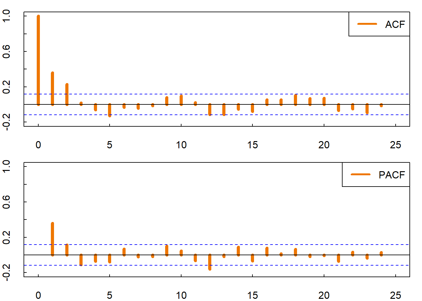

Estimation

ar1    <- arima(y,order=c(1,0,0))
ma1    <- arima(y,order=c(0,0,1))
ma2    <- arima(y,order=c(0,0,2))
arma11 <- arima(y,order=c(1,0,1))

# Information criteria
ar1_aic    <- (-2*ar1$loglik+2*3)/N     # (constant, phi, sigma_e)
ma1_aic    <- (-2*ma1$loglik+2*3)/N     # (constant, theta, sigma_e)
ma2_aic    <- (-2*ma2$loglik+2*4)/N     # (constant, theta1, theta2, sigma_e)
arma11_aic <- (-2*arma11$loglik+2*4)/N  # (constant, phi, theta, sigma_e)

ar1_bic    <- (-2*ar1$loglik+log(N)*3)/N
ma1_bic    <- (-2*ma1$loglik+log(N)*3)/N
ma2_bic    <- (-2*ma2$loglik+log(N)*4)/N
arma11_bic <- (-2*arma11$loglik+log(N)*4)/N

## table of likelihood and ICs
tab1 <- round( rbind( c(ar1$loglik,ma1$loglik.ma2$loglik,arma11$loglik), 
              c(ar1_aic,ma1_aic,ma2_aic,arma11_aic) , 
              c(ar1_bic,ma1_bic,ma2_bic,arma11_bic) ) ,  3 )
row.names(tab1) <- c("loglik", "AIC", "BIC")
colnames(tab1)  <- c("AR(1)", "MA(1)", "MA(2)", "ARMA(1,1)")
tab1

##           AR(1)    MA(1)    MA(2) ARMA(1,1)
## loglik -747.736 -746.702 -747.736  -746.702
## AIC       5.382    5.419    5.371     5.381
## BIC       5.421    5.458    5.423     5.433

Forecasting

## get forecasts
ar1_pred    <- predict(ar1, n.ahead=H)
ma1_pred    <- predict(ma1, n.ahead=H)
ma2_pred    <- predict(ma2, n.ahead=H)
arma11_pred <- predict(arma11, n.ahead=H)

## get fitted values
ar1_mu     <- y-ar1$residuals
ma1_mu     <- y-ma1$residuals
ma2_mu     <- y-ma2$residuals
arma11_mu  <- y-arma11$residuals

## compute RMSE
rmse <- function(y, f) {sqrt(mean((y-as.numeric(f))^2))}
ar1_mse    <-rmse(y.out, ar1_pred$pred)
ma1_mse    <-rmse(y.out, ma1_pred$pred)
ma2_mse    <-rmse(y.out, ma2_pred$pred)
arma11_mse <-rmse(y.out, arma11_pred$pred)

## Plot
par(mfrow = c(1,2))

myplot( dates[(N-10):(N+H)] , c(y[(N-10):N], y.out) , t='b', main=sprintf('AR(1) RMSE %3.3f',ar1_mse) , ylim=c(0,7) , col='darkorange' ) 
abline( v=dates[N] , lwd=2 )
abline( h=ar1$coef['intercept'] , lwd=2 )
lines( dates[(N-10):N] , ar1_mu[(N-10):N] , t='l' , lwd=2 , col='blue3' )
lines( dates[(N+1):(N+H)] , as.numeric(ar1_pred$pred)  , t='b' , lwd=2 , col='blue3' )

myplot( dates[(N-10):(N+H)] , c(y[(N-10):N], y.out) , t='b' , main=sprintf('ARMA(1,1) RMSE %3.3f',arma11_mse) , ylim=c(0,7) , col='darkorange' ) 
abline( v=dates[N] , lwd=2 )
abline( h=arma11$coef['intercept'] , lwd=2 )
lines( dates[(N-10):N] , arma11_mu[(N-10):N] , t='l' , lwd=2 , col='blue3' )
lines( dates[(N+1):(N+H)] , as.numeric(arma11_pred$pred)  , t='b' , lwd=2 , col='blue3' )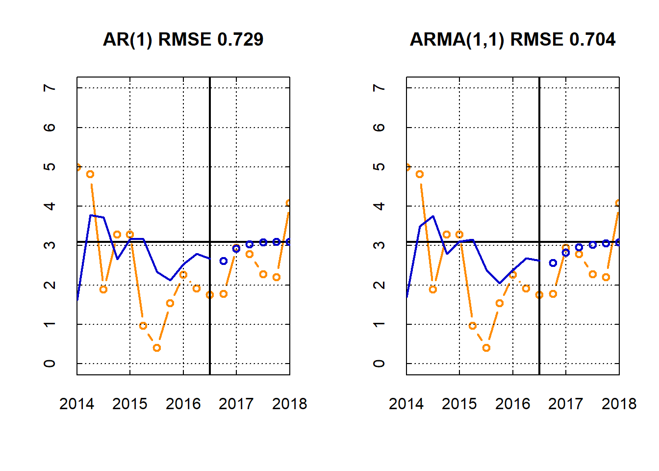

par(mfrow = c(1,2))

myplot( dates[(N-10):(N+H)] , c(y[(N-10):N], y.out) , t='b', main=sprintf('MA(2) RMSE %3.3f',ma2_mse) , ylim=c(0,7) , col='darkorange' ) 
abline( v=dates[N] , lwd=2 )
abline( h=ma2$coef['intercept'] , lwd=2 )
lines( dates[(N-10):N] , ma2_mu[(N-10):N] , t='l' , lwd=2 , col='blue3' )
lines( dates[(N+1):(N+H)] , as.numeric(ma2_pred$pred)  , t='b' , lwd=2 , col='blue3' )

myplot( dates[(N-10):(N+H)] , c(y[(N-10):N], y.out) , t='b' , main=sprintf('MA(1) RMSE %3.3f',ma1_mse) , ylim=c(0,7) , col='darkorange' ) 
abline( v=dates[N] , lwd=2 )
abline( h=ma1$coef['intercept'] , lwd=2 )
lines( dates[(N-10):N] , ma1_mu[(N-10):N] , t='l' , lwd=2 , col='blue3' )
lines( dates[(N+1):(N+H)] , as.numeric(ma1_pred$pred)  , t='b' , lwd=2 , col='blue3' )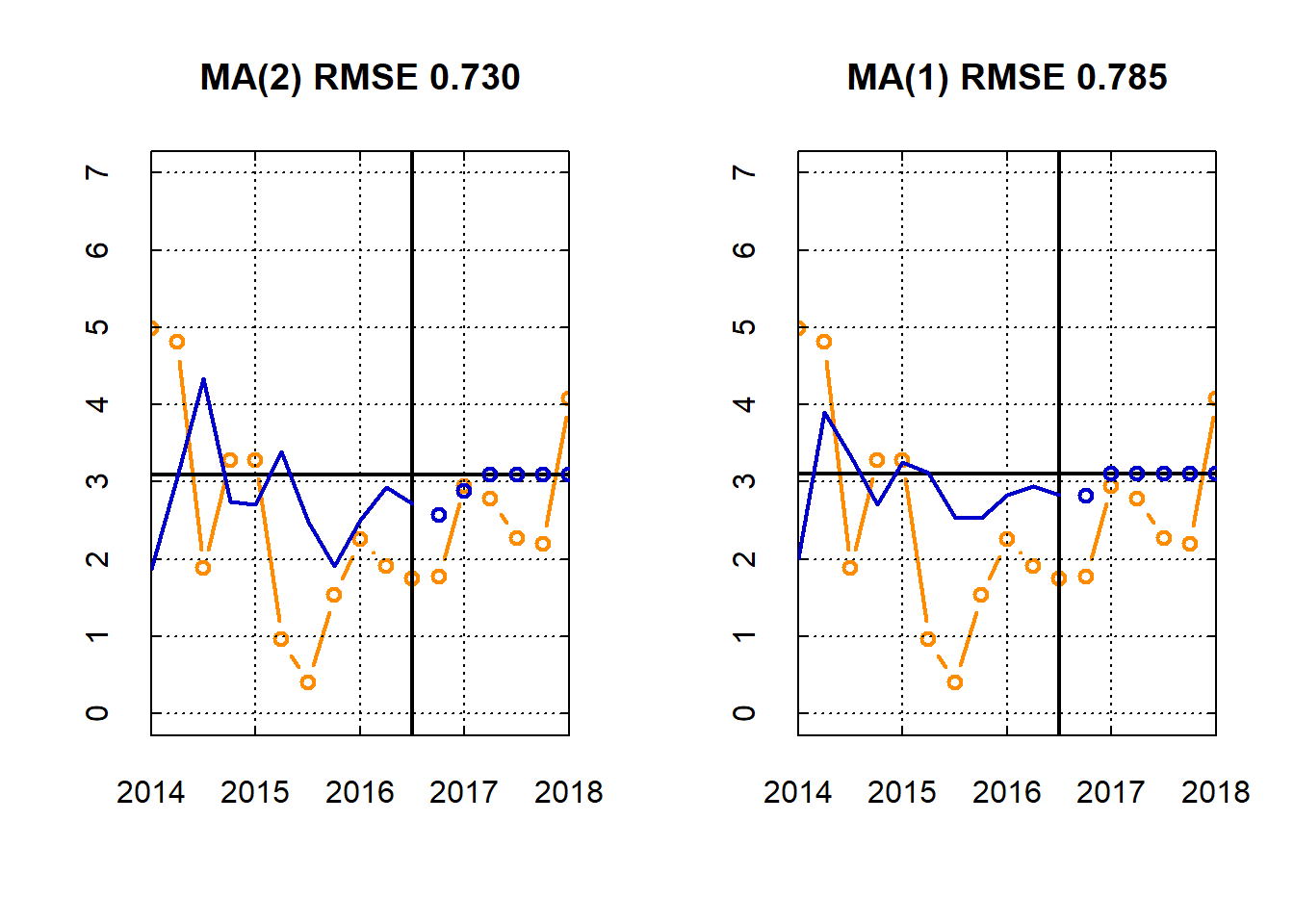

5.2 Exercises

Exercise 1 (Best forecast under the square loss)

Show that the best forecast under the square loss \[ L(y_{t+h}, \ \hat{y}_{t+h|t}) = (y_{t+h}-\hat{y}_{t+h|t})^2 \]

for some forecast horizon \(h \in \mathbb{N}\) is \[ \hat{y}_{t+h|t} = \mathbb{E} [y_{t+h} \ | \ y_t, \dots, y_1] \]

Exercise 2 (Best forecast under the absolute loss)

Show that the best forecast under the absolute loss \[ L(y_{t+h}, \ \hat{y}_{t+h|t}) = |y_{t+h}-\hat{y}_{t+h|t}| \]

for some forecast horizon \(h \in \mathbb{N}\) is \[ \hat{y}_{t+h|t} = \text{median}(y_{t+h} \ | \ y_t, \dots, y_1) \]

Exercise 3 (Invertibility of MA(1))

Consider the MA(1) process

\[ y_t = \theta \varepsilon_{t-1} + \varepsilon_t. \]

Show that:

if \(|\theta|<1\), then the process is invertible in the past observed values:

\[ \varepsilon_t = \sum_{j=0}^{\infty} (-\theta)^j y_{t-j} \]

if \(|\theta|>1\), then the process is invertible in the future observed values:

\[ \varepsilon_t = \frac{1}{\theta} \sum_{j=0}^{\infty} \left(-\frac{1}{\theta}\right)^j y_{t+j+1} \]